
Or how to get all your X from A to B for very little C. In this post I create an R implementation of optimizing a “minimum cost flow problem” in R using graph theory and the lpSolve package. This can be useful for transportation and allocation applications in supply chain, logistics, and planning.
The Problem
Recently I came across a business problem that I interpreted as a “minimum cost flow problem”. According to Wikipedia it is an optimization and decision problem to find the cheapest possible way of sending a certain amount of flow through a flow network. A typical application of this problem involves finding the best delivery route from a factory to a warehouse where the road network has some capacity and cost associated.
I was hoping for a readily available implementation of an algorithm for this problem via an R-package, but my search on CRAN did not yield any results. So I turned to StackOverflow. You can find my question here. Ultimately, I ended up answering it myself. If this is useful to you, I’d appreciate your upvote :)
Example
Let’s start off by building an example graph for illustrating the problem. I used a manually created edgelist, defining a directional graph. Each edge has a from node and a to node, given as numeric ID, as well as a capacity c (the maximum number of units that can pass through this connection), and a cost a (the cost of passing a single unit through this connection). The edgelist data frame can be turned into a graph object using the igraph package and its graph_from_edgelist function.
library(tidyverse)
library(igraph)
library(magrittr)

# create edgelist
edgelist <- data.frame(
  from = c(1, 1, 2, 2, 2, 3, 3, 3, 4, 4, 5, 5, 6, 6, 7, 8),
  to = c(2, 3, 4, 5, 6, 4, 5, 6, 7, 8, 7, 8, 7, 8, 9, 9),
  ID = seq(1, 16, 1),
  capacity = c(20, 30, 99, 99, 99, 99, 99, 99, 99, 99, 99, 99, 99, 99, 99, 99),
  cost = c(0, 0, 1, 2, 3, 4, 3, 2, 3, 2, 3, 4, 5, 6, 0, 0))

# make edgelist into graph object
g <- graph_from_edgelist(as.matrix(edgelist[,c('from','to')]))

# add properties
E(g)$capacity <- edgelist$capacity
E(g)$cost <- edgelist$cost

plot(g, edge.label = E(g)$capacity)
plot(g, edge.label = E(g)$cost)
The result looks like this:
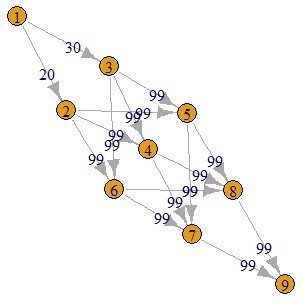
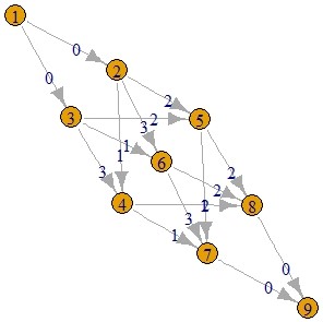
Note that the example I chose only uses non-standard capacities in the edges coming out of node 1, and only uses non-zero cost values in the edges of the middle layer. I separated cost and capacity out like that to keep it simple for this example. In a real world application the values are likely more mixed, and there would probably be a lot more edges.
With our example graph we are now ready to formulate the objective function and the constraints of our optimization. I use the function below to generate the inputs for our solver. They consist of a left-hand side lhs (a vector of integers representing coefficients of the flow through each edge), a direction dir (<, ==, >), and a right-hand side rhs giving the numeric value that will need to be met by each constraint.
The Solution
Our objective is to minimize the total cost incurred, subject to the relevant constraints
\[minimize(\sum_{i = 1}^{E} f(x_i) * c)\]Constraints are grouped into three major categories:
- capacity constraints: Flow f through any given edge x can’t be higher than the edge’s capacity c.
- node flow constraints: All units in our problem should pass the network. We cannot retain any units in the network, and we cannot have flow out of a node without the equivalent flowing in to that node as well. Therefore, the sum of units flowing through incoming nodes E(n) into a node needs to be exactly equal to the sum of units flowing through outgoing nodes E(o) out of that node.
- initialisation constraints: The node flow constraint is true for all except the source node s and the target node t. We are looking for a solution that pushes a fixed number of units from s through the network into t. Therefore, the sum of units flowing through the outgoing nodes E(s) out of s and the sum of units flowing through the incoming nodes E(t) into t needs to be exactly equal to that fixed number of units.
I have implemented all of that in the function below:
createConstraintsMatrix <- function(edges, total_flow) {

  # Edge IDs to be used as names
  names_edges <- edges$ID
  # Number of edges
  numberof_edges <- length(names_edges)

  # Node IDs to be used as names
  names_nodes <- c(edges$from, edges$to) %>% unique
  # Number of nodes
  numberof_nodes <- length(names_nodes)

  # Build constraints matrix
  constraints <- list(
    lhs = NA,
    dir = NA,
    rhs = NA)

  #' Build capacity constraints ------------------------------------------------
  #' Flow through each edge should not be larger than capacity.
  #' We create one constraint for each edge. All coefficients zero
  #' except the ones of the edge in question as one, with a constraint
  #' that the result is smaller than or equal to capacity of that edge.

  # Flow through individual edges
  constraints$lhs <- edges$ID %>%
    length %>%
    diag %>%
    set_colnames(edges$ID) %>%
    set_rownames(edges$ID)
  # should be smaller than or equal to
  constraints$dir <- rep('<=', times = nrow(edges))
  # than capacity
  constraints$rhs <- edges$capacity


  #' Build node flow constraints -----------------------------------------------
  #' For each node, find all edges that go to that node
  #' and all edges that go from that node. The sum of all inputs
  #' and all outputs should be zero. So we set inbound edge coefficients as 1
  #' and outbound coefficients as -1. In any viable solution the result should
  #' be equal to zero.

  nodeflow <- matrix(0,
                     nrow = numberof_nodes,
                     ncol = numberof_edges,
                     dimnames = list(names_nodes, names_edges))

  for (i in names_nodes) {

    # input arcs
    edges_in <- edges %>%
      filter(to == i) %>%
      select(ID) %>%
      unlist
    # output arcs
    edges_out <- edges %>%
      filter(from == i) %>%
      select(ID) %>%
      unlist

    # set input coefficients to 1
    nodeflow[
      rownames(nodeflow) == i,
      colnames(nodeflow) %in% edges_in] <- 1

    # set output coefficients to -1
    nodeflow[
      rownames(nodeflow) == i,
      colnames(nodeflow) %in% edges_out] <- -1
  }

  # But exclude source and target edges
  # as the zero-sum flow constraint does not apply to these!
  # Source node is assumed to be the one with the minimum ID number
  # Sink node is assumed to be the one with the maximum ID number
  sourcenode_id <- min(edges$from)
  targetnode_id <- max(edges$to)
  # Keep node flow values for separate step below
  nodeflow_source <- nodeflow[rownames(nodeflow) == sourcenode_id,]
  nodeflow_target <- nodeflow[rownames(nodeflow) == targetnode_id,]
  # Exclude them from node flow here
  nodeflow <- nodeflow[!rownames(nodeflow) %in% c(sourcenode_id, targetnode_id),]

  # Add nodeflow to the constraints list
  constraints$lhs <- rbind(constraints$lhs, nodeflow)
  constraints$dir <- c(constraints$dir, rep('==', times = nrow(nodeflow)))
  constraints$rhs <- c(constraints$rhs, rep(0, times = nrow(nodeflow)))


  #' Build initialisation constraints ------------------------------------------
  #' For the source and the target node, we want all outbound nodes and
  #' all inbound nodes to be equal to the sum of flow through the network
  #' respectively

  # Add initialisation to the constraints list
  constraints$lhs <- rbind(constraints$lhs,
                           source = nodeflow_source,
                           target = nodeflow_target)
  constraints$dir <- c(constraints$dir, rep('==', times = 2))
  # Flow should be negative for source, and positive for target
  constraints$rhs <- c(constraints$rhs, total_flow * -1, total_flow)

  return(constraints)
}

constraintsMatrix <- createConstraintsMatrix(edgelist, 30)
This should return something like this. We can see the rows corresponding to capacity constraints as lines with just a single 1 value in lhs, a <= in dir, and the capacity of the corresponding edge in the rhs. Node flow constraints show as one row per node, 1 for incoming nodes and -1 for outgoing nodes, == in dir, and zero in rhs. Finally, the initialisation constraints are implemented with negative coefficients for all edges leaving the source node and positive coefficients for all edges reaching the target node.
$lhs
1  2  3  4  5  6  7  8  9 10 11 12 13 14 15 16
1       1  0  0  0  0  0  0  0  0  0  0  0  0  0  0  0
2       0  1  0  0  0  0  0  0  0  0  0  0  0  0  0  0
3       0  0  1  0  0  0  0  0  0  0  0  0  0  0  0  0
4       0  0  0  1  0  0  0  0  0  0  0  0  0  0  0  0
5       0  0  0  0  1  0  0  0  0  0  0  0  0  0  0  0
6       0  0  0  0  0  1  0  0  0  0  0  0  0  0  0  0
7       0  0  0  0  0  0  1  0  0  0  0  0  0  0  0  0
8       0  0  0  0  0  0  0  1  0  0  0  0  0  0  0  0
9       0  0  0  0  0  0  0  0  1  0  0  0  0  0  0  0
10      0  0  0  0  0  0  0  0  0  1  0  0  0  0  0  0
11      0  0  0  0  0  0  0  0  0  0  1  0  0  0  0  0
12      0  0  0  0  0  0  0  0  0  0  0  1  0  0  0  0
13      0  0  0  0  0  0  0  0  0  0  0  0  1  0  0  0
14      0  0  0  0  0  0  0  0  0  0  0  0  0  1  0  0
15      0  0  0  0  0  0  0  0  0  0  0  0  0  0  1  0
16      0  0  0  0  0  0  0  0  0  0  0  0  0  0  0  1
2       1  0 -1 -1 -1  0  0  0  0  0  0  0  0  0  0  0
3       0  1  0  0  0 -1 -1 -1  0  0  0  0  0  0  0  0
4       0  0  1  0  0  1  0  0 -1 -1  0  0  0  0  0  0
5       0  0  0  1  0  0  1  0  0  0 -1 -1  0  0  0  0
6       0  0  0  0  1  0  0  1  0  0  0  0 -1 -1  0  0
7       0  0  0  0  0  0  0  0  1  0  1  0  1  0 -1  0
8       0  0  0  0  0  0  0  0  0  1  0  1  0  1  0 -1
source -1 -1  0  0  0  0  0  0  0  0  0  0  0  0  0  0
target  0  0  0  0  0  0  0  0  0  0  0  0  0  0  1  1

$dir
[1] "<=" "<=" "<=" "<=" "<=" "<=" "<=" "<=" "<=" "<=" "<=" "<=" "<=" "<="
[15] "<=" "<=" "==" "==" "==" "==" "==" "==" "==" "==" "=="

$rhs
[1]  20  30  99  99  99  99  99  99  99  99  99  99  99  99  99  99   0
[18]   0   0   0   0   0   0 -30  30
We can now feed all of this information to lpSolve to calculate the optimal flow values of each edge. Our example is relatively small, but because all values are integers it will compile relatively fast, even for much larger number of edges. I have successfully run a similar version of this code for a network with several thousands of edges in less than a minute on my laptop.
library(lpSolve)

# Run lpSolve to find best solution
solution <- lp(
  direction = 'min',
  objective.in = edgelist$cost,
  const.mat = constraintsMatrix$lhs,
  const.dir = constraintsMatrix$dir,
  const.rhs = constraintsMatrix$rhs)

# Print vector of flow by edge
solution$solution
Visualising the Output
To finish off, we write the resulting solution back to the igraph object and visualise the flow in the optimal solution in a plot
E(g)$flow <- solution$solution

# Get some colours in to visualise cost
E(g)$color[E(g)$cost == 0] <- 'royalblue'
E(g)$color[E(g)$cost == 1] <- 'yellowgreen'
E(g)$color[E(g)$cost == 2] <- 'gold'
E(g)$color[E(g)$cost >= 3] <- 'firebrick'

# Flow as edge size,
# cost as colour
plot(g, edge.width = E(g)$flow)
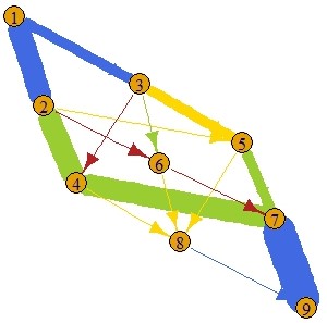
As you can see, the flow from node 1 is split between edges 1 and 2 because of the limiting capacity, even though this means that some of the flow will have to go from node 3 to node 5 at a higher cost. Expensive edges are avoided all together and have zero flow.
That’s all for now, thanks for reading! I hope it is helpful for someone out there. If you have any comments, questions, or suggestions, please send me an email or tweet. Any feedback would be much appreciated.