R Dataframes in the tidyverse are more than just simple tables these days. They can store complex information in list columns, and this becomes an immensely powerful framework when we use it to apply methods to different sets of data in parallel. In this article I illustrate this approach using data for a rare UK bird species to investigate if its distribution has been impacted by climate change.

Motivation

After recently seeing a Hadley Wickham lecture on nested models I became incredibly excited about nested dataframes with s3 objects in list columns again. Here is the video I am talking about:

Hadley uses this approach for data exploration but I think it is also very powerful for iterative workflows and for experimentation or hypothesis testing on large datasets. For example, when working on my PhD thesis I was routinely fitting hundreds of machine learning models at once. All models used the same predictor set and only varied in hyperparameters as well as label data. Yet, I had to run them in separate parallel processes and load the data into each of these. Moreover, when capturing results I often looked to the list class for help. This did the job but also meant that I had to be very careful about which results belonged to which data, which hyperparameters, and which model object.

Enter nested dataframes. They still rely on the list class, but they nicely organise the corresponding data elements together, in accordance with the tidy data framework

Data

I decided to explore this framework hands-on, using a small exemplary case study in the domain of species distribution modelling. This is what the models I mentioned earlier were. For this type of modelling task we need species occurrence data (our “label”, “response”, or Y) and climatic variables (the “predictors”, or X)

Species Data

After browsing the web for a suitable case study species for a while I decided on the Scottish Crossbill (Loxia scotica). This is a small passerine bird that inhabits the Caledonian Forests of Scotland, and is the only terrestrial vertebrate species unique to the United Kingdom. Only ~ 20,000 individuals of this species are alive today.

Getting species occurrence data used to be the main challenge in Biogeography. Natural Historians such as Charles Darwin and Alexander von Humboldt would travel for years on rustic sail ships around the globe collecting specimen. Today, we are standing on the shoulders of giants. Getting data is fast and easy thanks to the work of two organisations:

• the Global Biodiversity Information Facility (GBIF), an international network and research infrastructure funded by the world’s governments and aimed at providing anyone, anywhere, open access to data about all types of life on Earth. We will use their data in this project.

• rOpenSci, a non-profit initiative that has developed an ecosystem of open source tools, runs annual unconferences, and reviews community developed software. They provide an R package called rgbif that I once made a humble contribution to. It is essentially a wrapper around the GBIF API will help us access the species data straight into R.

library(tidyverse)
library(rgbif)

# get the database id ("key") for the Scottish Crossbill
speciesKey <- name_backbone('Loxia scotica')$speciesKey

# get the occurrence records of this species
gbif_response <- occ_search(
  scientificName = "Loxia scotica", country = "GB",
  hasCoordinate = TRUE, hasGeospatialIssue = FALSE,
  limit = 9999)

# backup to reduce API load
write_rds(x = gbif_response, path = here::here('gbif_occs_loxsco.rds'))

GBIF and rOpenSci just saved us years or roaming around the highlands with a pair of binoculars, camping in mud, rain, and snow, and chasing crossbills through the forest. Nevertheless, it is still up to us to make sense of the data we got back, in particular to clean it, as data collected on this large scale can have its own issues. Luckily, GBIF provides some useful metadata on each record. Here, I will exclude those that

• are not tagged as “present” (they may be artifacts from collections)
• don’t have any flagged issues (nobody has noticed anything abnormal with this)
• are under creative commons license (we can use them here)
• are older than 1965

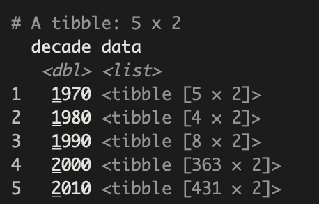
After cleaning the data we use tidyr::nest() to aggregate the data by decade.

library(lubridate)
birds_clean <- gbif_response$data %>%
  # get decade of record from eventDate
  mutate(decade = eventDate %>% ymd_hms() %>% round_date("10y") %>% year() %>% as.numeric()) %>%
  # clean data using metadata filters
  filter(
    # only creative commons license records
    str_detect(license, "http://creativecommons.org/") &
    # only records with no issues
    issues == "" &
    # no records before 1965
    decade >= 1970 &
    # no records after 2015 (there is not a lot of data yet)
    decade < 2020) %>%
  # retain only relevant variables
  select(decimalLongitude, decimalLatitude, decade) %>% arrange(decade)

birds_nested <- birds_clean %>%
  # define the nesting index
  group_by(decade) %>%
  # aggregate data in each group
  nest()

# let's have a look
glimpse(birds_nested)

Climate data

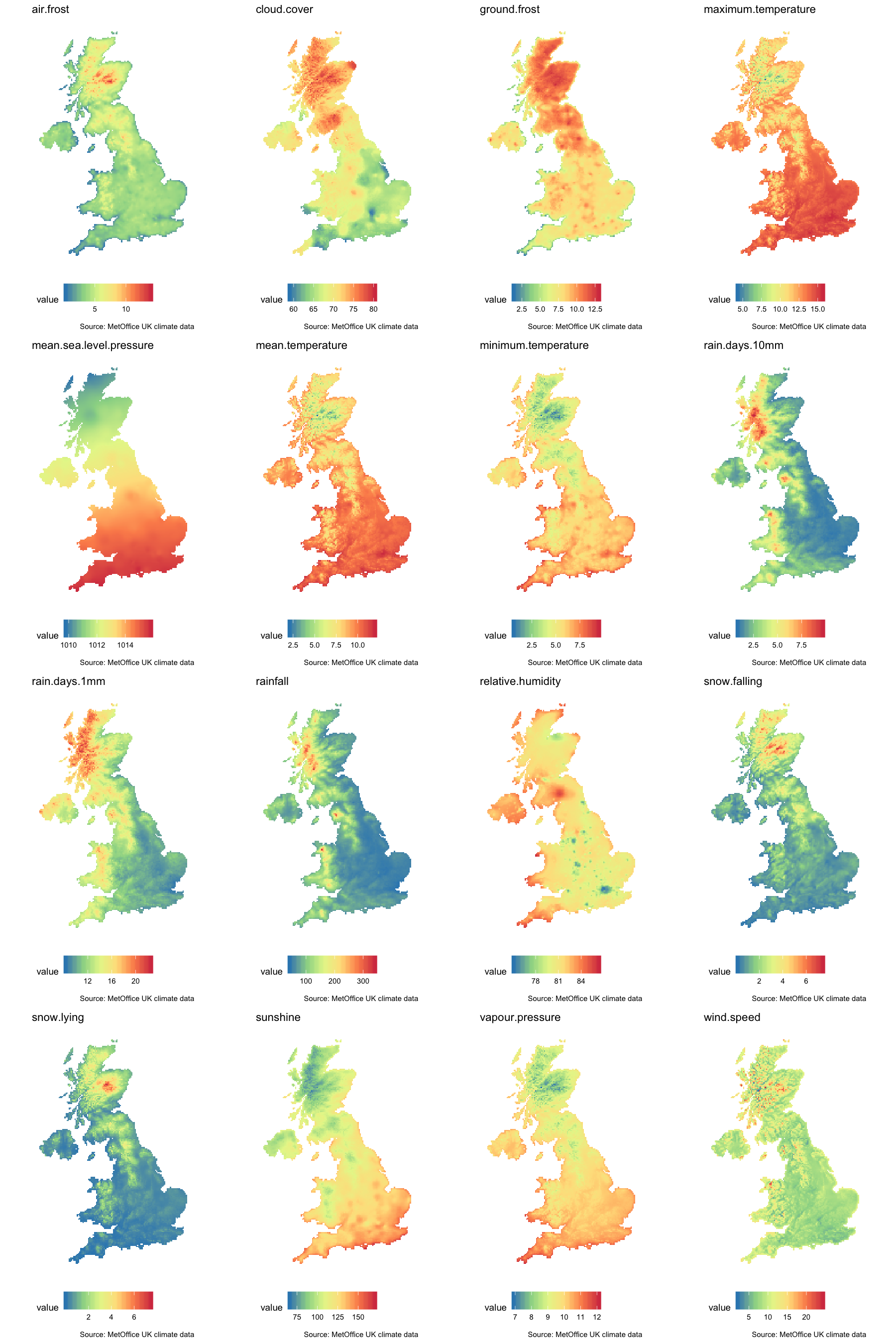
For the UK the MetOffice had some nice climatic datasets available. They were in a horrible format (CSV with timesteps, variable types, and geospatial information spread across rows, columns, and file partitions) but I managed to transform them into something useable. The details of this are beyond the scope of this post, but if you are interested in the code for that you can check it out here.

The final rasters look like this:

Modelling

We’ll split the data in training and test set with a true temporal holdout from all data collected between 2005 - 2015.

# last pre-processing step
df_modelling <- df_nested %>%
  # get into modelling format
  unnest() %>%
  # caret requires a factorial response variable for classification
  mutate(presence = case_when(
    presence == 1 ~ "presence",
    presence == 0 ~ "absence") %>%
    factor()) %>%
  # drop all observations with NA variables
  na.omit()

# create a training set for the model build
df_train <- df_modelling %>%
  # true temporal split as holdout
  filter(decade != "2010") %>%
  # drop decade, it's not needed anymore
  dplyr::select(-decade)

# same steps for test set
df_test <- df_modelling %>%
  filter(decade == "2010") %>%
  dplyr::select(-decade)

Species responses to environmental variables are often non-linear. For example, a species usually can’t survive if it is too cold, but it can’t deal with too much heat either. It needs the “sweet spot” in the middle. Linear models like a glm are not very useful under these circumstances. On the other hand, algorithms such as random forest can easily overfit to this kind of data. I therefore decided to test a regularised random forest (RFF) as introduced by Deng (2013), hoping that it would offer just the right ratio of bias vs variance for this use case.

Caret makes the model fitting incredibly easy! All we need to do is specify a tuning grid of hyperparameters that we want to optimise, a tune control that adjusts the number of iterations and the loss function used, and then call train with the algorithm we have picked.

library(RRF)

# for reproducibility
set.seed(12345)

# set up model fitting parameters
# tuning grid, trying every possible combination
tuneGrid <- expand.grid(
  mtry = c(3, 6, 9),
  coefReg = c(.01, .03, .1, .3, .7, 1),
  coefImp = c(.0, .1, .3, .6, 1))
tuneControl <- trainControl(
  method = 'repeatedcv',
  classProbs = TRUE,
  number = 10,
  repeats = 2,
  verboseIter = TRUE,
  summaryFunction = twoClassSummary)
# actual model build
model_fit <- train(
  presence ~ .,
  data = df_train,
  method = "RRF",
  metric = "ROC",
  tuneGrid = tuneGrid,
  trControl = tuneControl)

plot(model_fit)

We can evaluate the performance of this model on our hold-out data from 2005 - 2015. Just as uring training we are using the Area under the Receiver Operator Characteristic curve (AUC). With this metric, a model no bettern than random would score 0.5 while a perfect model making no mistakes would score 1.

# combine prediction with validation set
df_eval <- data_frame(
  "obs" = df_test$presence,
  "pred" = predict(
    object = model_fit,
    newdata = df_test,
    type = "prob") %>%
    pull(1))

# get ROC value
library(yardstick)
roc_auc_vec(estimator = "binary", truth = df_eval$obs, estimate = df_eval$pred)

Now we can combine the raw data, model performance, and predictions all in one nested dataframe. We can save this for later to make sure we always know what data was used to build which model.

df_eval <- df_modelling %>%
  group_by(decade) %>% nest() %>%
  # combine with climate data
  left_join(climate_nested, by = "decade") %>%
  # evaluate by decade
  mutate(
    "obs" = map(
      .x = data,
      ~ .x$presence),
    "pred" = map(
      .x = data,
      ~ predict(model_fit, newdata = .x, type = "prob") %>% pull("presence")),
    "auc" = map2_dbl(
      .x = obs,
      .y = pred,
      ~ roc_auc_vec(
          estimator = "binary",
          truth = .x,
          estimate = .y)),
    "climate_data" = map(
      .x = raster_stacks,
      ~ as(.x, "SpatialPixelsDataFrame") %>%
        as_data_frame() %>%
        na.omit()),
    "habitat_suitability" = map(
      .x = climate_data,
      ~ predict(model_fit, newdata = .x, type = "prob") %>% pull("presence"))
    )

df_eval

Conclusion

Let’s look at the change over time using gganimate. Unfortunately, we can see that the suitable area for the species in the UK is drastically decreasing after 1985. Not all species are negatively affected by climate change but many are. And this is just one of the many unintended consequences of our impact on planet earth.

I hope that you enjoyed this blog post despite our pessimistic findings. As you can see nested dataframes with list columns are immensely powerful in a range of situations. I will certainly use them a lot more in the future. Please let me know in the comments if you are, too!