
This post is an event report and a quick walk through to a submission that I developed with a group of participants at an Alibaba / Met Office UK hackathon. We are using the A* algorithm with a couple of tweaks to route cargo balloons from London to a number of cities in the UK.
It’s the year 2050. The invention of anti-gravity engines has led to the creation of unmanned balloons that travel the UK, delivering goods. However, unpredictable weather conditions mean that these balloons are often delayed, damaged or even destroyed(!), so we need your help. We’re inviting you to join our contest AND our hackathon to create an algorithm which allows these balloons to get to their route safely and effectively.
In January of this year, the Met Office teamed up with Alibaba Cloud in organising a hackathon at Huckletree Shoreditch. Here is a short video that gives a good impression of the event
The Problem
The hackathon was organised as a “Future Challenge”, a fictitious scenario for the year 2050. Obviously, drone delivery would be considered so 2020 and completely outdated by then. Instead, people are relying on anti-gravity balloons to deliver goods to cities across the UK via air drop. These anti-gravity balloons are reliable and efficient, but have one major shortcoming: They crash when travelling in areas with high wind speeds. This is where the Met Office comes in. The task was to navigate balloons from origin to destination while avoiding storms by using the Met Office forecasts.
I’ll spare you the full run through of rules, terms, and conditions. You can find them on the competition page. The main facts:
- forecast data provides projected wind speed for fields of a grid
- forecasts are for hourly intervals
- balloons can move up, down, left, right, or stay in place
- balloons move one field per 2 minutes
- balloons crash when entering a field when the wind speed is ≥15
So the big question is: How do we safely get the balloons from origin to destination while avoiding stormy areas? I teamed up with a nice bunch of people, mostly undergrad or master level university students. It was great to see their enthusiasm for working on this problem!
The Data
The data that was provided to us was:
- the coordinates of cities (origin and destinations)
- weather data, separated into: * a training set with 7 days of weather forecasts from 10 models plus observations of the actual conditions that manifested on these days * a holdout set with 5 days of weather forecasts
You should still be able to get the data here in case you’d like to have a go yourself. Note that the weather forecasts came in at a rather inconvenient file size of 2 x 800 MB, and download speeds were not that great either.
See the map below for illustration purposes. The map shows gridded forecasts of wind speed for a one hour time slice, as well as city locations (origin in yellow, destinations in red). Weather Forecast
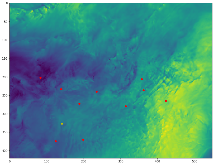
Weather Prediction
We started by looking at the weather predictions. Our initial plan was to use the first week, for which both forecasts and observations were available, to train a classifier that would identify the likelihood of high wind speeds in a given area at a particular time. This, however, turned out to be a bit of a red herring. The Met Office predictions were so good that averaging them and using a simple threshold of 15 resulted in close to zero false negatives when trying to detect cells with storms.
Lesson learned: Do your EDA properly to check which areas are worth investigating in detail and where you can use a simple ad-hoc solution.
import numpy as np
import pandas as pd
import matplotlib.pyplot as plt
import h5py

def convert_forecast(data_cube):
    # take mean of forecasts
    arr_world = np.min(data_cube, axis=2)
    # binarize to storm (1) or safe (0)
    arr_world = arr_world >= 15
    # from boolean to binary
    arr_world = arr_world.astype(int)
    # swap axes so x=0, y=1, z=2, day=3
    arr_world = np.swapaxes(arr_world,0,2)
    arr_world = np.swapaxes(arr_world,1,3)
    arr_world = np.swapaxes(arr_world,2,3)

    return(arr_world)

data_cube = np.load('../data/5D_test.npy')
# convert forecast to world array
forecast = convert_forecast(data_cube)
Balloon Navigation
We wanted balloons to take the shortest path from origin to destination without passing into storms. That means storms can be viewed as obstacles in our path search problem, because we would never, ever, want to pass through them, even if that means a massive detour for the balloon. We therefore chose to use an A* path search algorithm. This algorithm finds the shortest path around obstacles in a reasonable amount of time and is quite straight forward to implement.
The basic approach is to start from origin and generate a frontier possible next moves from a list of valid neighbouring fields. Fields with obstacles are excluded, as well as fields that have been visited before. For each field that is part of this frontier we log which field we came from and calculate a heuristic cost of our movement to far. As soon as the destination field becomes part of the frontier, we can recursively follow the trail laid out in our log, back to the origin, to find the shortest path.
In case you would like more details or want to compare A* to other pathfinding algorithms, this page has the best summary of pathfinding algorithms I have seen, including a great section on A* with interactive simulations.
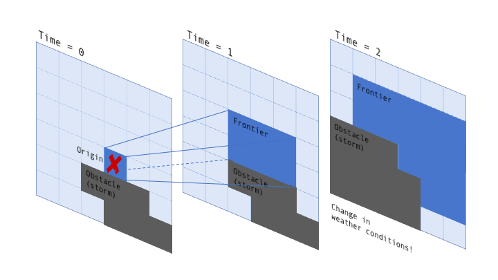
In our case, there is one additional complication: our search is two-dimensional (geographical space with latitude and longitude), but our “obstacles” change over time. My way around that was to make the search three-dimensional, with each movement time step (2 minutes) as a slice in the third dimension.
# repeat time slices x30
forecast_stack = np.repeat(forecast, repeats=30, axis=2)
I then forced the search algorithm
to always take a step forward in time by restricting the valid neighbours to
[..., ..., z+1]. I tried to illustrate this schematically in the diagramm below:
The code for my A* implementation in python using heapq can be found below.
Note that I allow for neighbours that have the same x and y coordinates. This essentially allows balloons to “hover in place” to wait out unfavourable weather conditions in the area ahead, should that be the most promising course of action.
Another thing to mention is that this approach massively inflates our frontier.
Usually, an advantage of the A* algorithm is that fields that have been visited
before do not need to be considered again. In my approach, field [0,0,0] is
different from field [0,0,1] (the same latitude and longitude, but a different
time step). As a result, computation becomes a lot more resource intense, but it
is still feasible to run this on your local machine and in the fast-paced
setting of a hackathon I think that prioritising developer time over computing
time was the right call.
import heapq

def heuristic_function(a, b):
    return (b[0] - a[0]) ** 2 + (b[1] - a[1]) ** 2

def astar_3D(space, origin_xy, destination_xy):
    # make origin 3D with timeslice 0
    origin = origin_xy[0], origin_xy[1], 0
    # logs the path
    came_from = {}
    # holds the legal next moves in order of priority
    frontier = []
    # define legal moves:
    # up, down, left, right, stay in place.
    # no diagonals and always move forward one time step (z)
    neighbours = [(0,0,1),(0,1,1),(0,-1,1),(1,0,1),(-1,0,1)]

    cost_so_far = {origin: 0}
    priority = {origin: heuristic_function(origin_xy, destination_xy)}
    heapq.heappush(frontier, (priority[origin], origin))

    # While there is still options to explore
    while frontier:

        current = heapq.heappop(frontier)[1]

        # if current position is destination,
        # break the loop and find the path that lead here
        if (current[0], current[1]) == destination_xy:
            data = []
            while current in came_from:
                data.append(current)
                current = came_from[current]
            return data

        for i, j, k in neighbours:
            move = current[0] + i, current[1] + j, current[2] + k

            # check that move is legal
            if ((0 <= move[0] < space.shape[0]) &
                (0 <= move[1] < space.shape[1]) &
                (0 <= move[2] < space.shape[2])):

                if space[move[0], move[1], move[2]] != 1:

                    new_cost = 1
                    new_total = cost_so_far[current] + new_cost

                    if move not in cost_so_far:
                        cost_so_far[move] = new_total
                        # calculate total cost
                        priority[move] = new_total + heuristic_function(move, destination_xy)
                        # update frontier
                        heapq.heappush(frontier, (priority[move], move))
                        # log this move
                        came_from[move] = current

    return 'no solution found :('

# get city data
cities = pd.read_csv('../data/CityData.csv', header=0)
# run algorithm
x = astar_3D(space=arr_world_big[:,:,:,0],
             origin_xy=origin,
             destination_xy=destination)
Visualising the Results
We have a predicted optimal route now. That’s great, but it would be even
better to visualise these results in a way that allows us to develop some
intuition about how our solution is doing and where we could improve it further.
I thought that an animation of the time slices with the paths generated would
be ideal for this. So I used matplotlib.pyplot to create an image of each
time slice and then combined them into an animated gif. Output and code below:
You can see that, for this day, the solution for most cities is relatively straight-forward because of low wind speeds in the majority of the area. However, the A* pathfinding algorithm can be seen nicely at work in the later timeslices and the centre-right of the map, where the purple balloon pauses for a timeslice to wait out unfavourable conditions ahead and then winds around patches of high wind speed towards its target.
def plot_solution(world, cities, solution, day):
    timesteps = list(range(0, 540, 30))
    solution = solution.loc[solution.day == day,:]
    # colour map for cities
    cmap = plt.cm.cool
    norm = matplotlib.colors.Normalize(vmin=1, vmax=10)
    # colour map for weather
    cm = matplotlib.colors.LinearSegmentedColormap.from_list('grid', [(1, 1, 1), (0.5, 0.5, 0.5)], N=2)

    for t in timesteps:
        timeslice = world[:,:,t]
        moves_sofar = solution.loc[solution.z <= t,:]
        moves_new = solution.loc[(t <= solution.z) & (solution.z <= t + 30),:]

        if len(solution_subset) > 0:
            plt.figure(figsize=(5,5))
            plt.imshow(timeslice[:,:].T, aspect='equal', cmap = cm)

            # plot old moves
            for city in moves_sofar.city.unique():
                moves_sofar_city = moves_sofar.loc[moves_sofar.city == city,:]
                x = moves_sofar_city.x
                y = moves_sofar_city.y
                z = moves_sofar_city.z
                plt.plot(list(x), list(y), linestyle='-', color='black')

            # plot new moves
            for city in moves_new.city.unique():
                moves_new_city = moves_new.loc[moves_new.city == city,:]
                x = moves_new_city.x
                y = moves_new_city.y
                z = moves_new_city.z
                plt.plot(list(x), list(y), linestyle='-', color=cmap(norm(city)))

            # plot cities
            for city,x,y in zip(cities.cid, cities.xid, cities.yid):
                if city == 0:
                    plt.scatter([x-1], [y-1], c='black')
                else:
                    # balloon still en-route?
                    if city in moves_new.city.unique():
                        plt.scatter([x-1], [y-1], c=cmap(norm(city)))
                    else:
                        plt.scatter([x-1], [y-1], c='black')

            # save and display
            plt.savefig('img_day' + str(day) + '_timestep_' + str(t) + '.png')
            plt.show()