
Here I summarise learnings from lesson 1 of the fast.ai course on deep learning. fast.ai is a deep learning online course for coders, taught by Jeremy Howard. Its tag line is to “make neural nets uncool again”. I started the class a couple of days ago and have been impressed with how fast it got me to apply the methods, an approach described by them as top-down learning. I am writing this blog post to document and reflect on the things that I learned and to help other people that may be interested getting started with the class.
The fast.ai library is a high-level library based on PyTorch, which tries to take a selection of best-practice approaches from cutting edge deep learning research and make them into a collection of intelligent default settings.
Lesson 2 outlined the fundamentals of computer vision and building image classification models. My homework: get my hands on my own image dataset and use it to train a classifier myself. I chose to attempt a classifier that can distinguish between sharks and dolphins, using images from google image search. Read along for a detailed walk through below.
Getting an Image Dataset
This handy tool allows us to get images directly from google image search.
$ pip install google_images_download
For more than 100 images we also need to install chromedriver and dependencies:
$ apt-get install python-selenium python3-selenium libxi6 libgconf-2-4 chromium-chromedriver
Note that I had some problems with accessing the chrome driver from jupyter
notebooks. Changing ownership of the file with
chmod 777 /usr/local/bin/chromedriver
solved this for me.
Now we can run a query for images. Results are named as the number of the result
plus the original file name, downloaded, and saved locally. Note that you
should make sure to utilise the usage_rights flag in order to get images
that are cleared for this type of use.
from google_images_download import google_images_download

os.chdir('/home/paperspace/data/sharksdolphins/')
response = google_images_download.googleimagesdownload()

arguments = {
 "keywords": '"shark","dolphin"',
 "print_urls": False,
 "limit": "10000",
 "output_directory": "sharksdolphins/train/",
 "format": "jpg",
 "usage_rights": "labeled-for-nocommercial-reuse",
 "chromedriver": "/usr/local/bin/chromedriver"
}

response.download(arguments)

# func for renaming an image file
def image_rename(file):
    file_index = re.match(r'\A\d*', file).group(0)
    file_index = file_index.zfill(3)
    return file_index+'.jpg'

# func for renaming all files in a folder
def image_rename_all(folder):
    files = os.listdir(folder)
    [os.rename(folder+file, folder+image_rename(file)) for file in files]

# rename files
folders = ['data/sharksdolphins/train/shark/',
           'data/sharksdolphins/train/dolphin/']
[image_rename_all(folder) for folder in folders]
The above query returned about 800 images each. I ended up speeding through these images manually and removing unsuitable images manually.
We need a training and a validation set. Making this work with fast.ai is easily
done by adapting the recommended folder structure of a data folder with two
sub-folders (train and valid), each of which have a subfolder with images
for each class.
The code chunk below takes the images downloaded earlier and randomly splits them into 80% training data and 20% validation data. Don’t forget to set a random seed so that your results stay reproducible.
# split files into test and training set# split
PATH = 'data/sharksdolphins/'
files_sharks = os.listdir(f'{PATH}train/shark')
files_dolphins = os.listdir(f'{PATH}train/dolphin')

# sample from each class to create a validation set
np.random.seed(1234)
files_sharks_val = np.random.choice(
    files_sharks,
    size=round(len(files_sharks) / 5),
    replace=False,
    p=None)
files_dolphins_val = np.random.choice(
    files_dolphins,
    size=round(len(files_dolphins) / 5),
    replace=False,
    p=None)

# move validation set images into validation folder
[os.rename(PATH+'train/shark/'+file, PATH+'valid/shark/'+file)
  for file in files_sharks_val]
[os.rename(PATH+'train/dolphin/'+file, PATH+'valid/dolphin/'+file)
  for file in files_dolphins_val]
As you will see, collecting the data was the hardest part and everyting from here onward is quite straight-forward thanks to the high level abstractions provided by fast.ai
Training a Model
Now we can finally start to train our image classifier. I am using a paperspace instance with the setup recommended and provided by fast.ai.
Train a First Model
os.chdir('/home/paperspace/')
# append fast.ai local folder to system path so modules can be imported
sys.path.append('/home/paperspace/fastai/')
# automatically reload updated sub-modules
%reload_ext autoreload
%autoreload 2
# in-line plots
%matplotlib inline

from fastai.imports import *
from fastai.transforms import *
from fastai.conv_learner import *
from fastai.model import *
from fastai.dataset import *
from fastai.sgdr import *
from fastai.plots import *
# set path of data folder
PATH = "data/sharksdolphins/"
# set size images should be resized to
sz = 224
# First model
arch = resnet34
data = ImageClassifierData.from_paths(PATH, tfms=tfms_from_model(arch, sz), bs=16)
learn = ConvLearner.pretrained(arch, data, precompute=True)
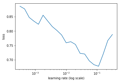
Jeremy explained the learning rate finder that uses the approach of cyclical
learning rates as outlined by Leslie Smith (https://arxiv.org/abs/1506.01186).
Using the lr_find method and then plotting the learning rate against loss.
We now want to visually choose the “The highest learning rate we can find where
the loss is still clearly improving”. Note here that the learning rate finder
did initially not work so well for my small-ish dataset. I had to adjust the
batch size to make it work correctly
(see bs=16 argument in the ImageClassifierData call above)
learn.lr_find()
learn.sched.plot_lr()
learn.fit(0.01, 5)
| epoch | trn_loss | val_loss | accuracy |
|---|---|---|---|
| 0 | 0.435999 | 0.267501 | 0.925 |
| 1 | 0.3081 | 0.29459 | 0.9 |
| 2 | 0.2548 | 0.235716 | 0.925 |
| 3 | 0.214654 | 0.229093 | 0.93125 |
| 4 | 0.237024 | 0.162347 | 0.9375 |
Over 93% accuracy! Really nice results already!
Let’s see if we can improve things even further.
Train a Second Model
Now let’s start training some of the lower layers and retraining these with differential learning rate. Jeremy talks about unfreezing here, but a friend that I talked to about this called it thawing instead, and I like that terminology, as it implies the differential learning rates with fast-changing weights at the last layer but slower updates in the lower layers.
# unfreeze pretrained layers
learn.unfreeze()
# set differential learning rate
lr = np.array([1e-4,1e-3,1e-2])
# train new model
learn.fit(lr, 3, cycle_len=1, cycle_mult=2)
| epoch | trn_loss | val_loss | accuracy |
|---|---|---|---|
| 0 | 0.475365 | 0.365881 | 0.89375 |
| 1 | 0.278049 | 0.177107 | 0.94375 |
| 2 | 0.174708 | 0.178467 | 0.95 |
| 3 | 0.120919 | 0.230777 | 0.95625 |
| 4 | 0.093978 | 0.148054 | 0.95625 |
| 5 | 0.081571 | 0.200582 | 0.95 |
| 6 | 0.055903 | 0.198029 | 0.95 |
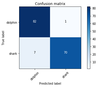
A little bit better yet. Let’s look at the confusion matrix and some of the misclassified images:
# get predictions and transform to class probability values
log_preds = learn.predict()
preds = np.argmax(log_preds, axis=1)
probs = np.exp(log_preds[:,1])

# plot confusion matrix
from sklearn.metrics import confusion_matrix
cm = confusion_matrix(data.val_y, preds)
plot_confusion_matrix(cm, data.classes)
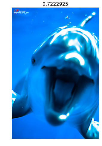
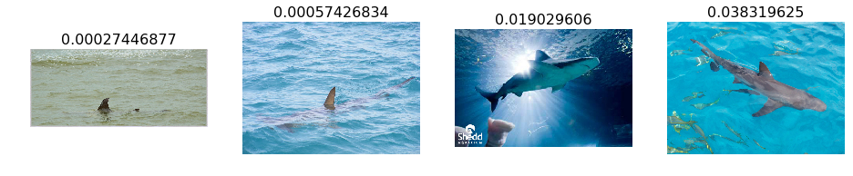
We should also plot some of the images to develop an intuition about where our classifier does well and where it doesn’t. Here is the one misclassified dolphin and the top 4 misclassified sharks:
Discussion
You can see that we got some pretty strong results in a very short amount of time and using a very limited dataset! There is obviously many more things that could be done to improve this model further.
Weighting the Classes
In our example of sharks and dolphins, we are currently treating all misclassifications equally. This may not be the right approach! If the model was used to monitor a beach for sharks, for example, failing to recognize a dolphin would not be a problem, while failing to recognize a shark could potentially result in human fatalities. In this case, it might be advisable to retrain the model with a biased weighting function to make sure our recall on shark images is higher.
Data Leakage
Looking at images that were misclassified or low-confidence predictions, I realised that my training set introduced a number of hidden biases to the model. For example, a number of dolphin pictures have people in them that are touching the dolphin. This is less prevalent with the shark pictures, for obvious reasons. As a result, the few shark pictures with human arms and hands in them and near the shark seem to end up with lower confidence for the shark class. For the only misclassified dolphin in the dataset, on the other hand, I think that the shark-like pose (frontal, widely opened mouth) may have played a role in the model mistaking this image for a shark image.
This kind of data leakage is increasingly discussed and criticised in deep learning applications, so it is good to be aware and keep an eye out for them. Since my model is not going into production for Baywatch any time soon, I am just glad I found it nicely illustrated in this relatively small dataset.